class: ur-title, center, middle, title-slide # BST430 Lecture 5a ## Reshaping and combining data frames ### Andrew McDavid ### U of Rochester ### 2021-09-06 (updated: 2021-09-15) --- ## Agenda 1. Reshaping a single data frame 2. Joining multiple data frames ## Announcements 1. Office hours Friday moved to noon (or by appointment) and will be virtual. <br> 1. Make sure that you don't have any "M" status in your homework 1 -- these are files with modifications that haven't been pushed to github. I have observed that some people haven't pushed the .md files. 2. If you are having troubles, I am available for consult after class. 3. Remember that you can always make corrections to an assignment for partial credit. --- class: middle # .hand[We...] .huge[.green[have]] .hand[unformatted or untidy data] .huge[.pink[want]] .hand[to reorganize the data to carry on with our analysis] --- class: code50 ## Data: Sales <br> .pull-left[ ### .green[We have...] .code50[ ``` ## # A tibble: 2 × 4 ## cust_id item_1 item_2 item_3 ## <dbl> <chr> <chr> <chr> ## 1 1 bread milk banana ## 2 2 milk toilet paper <NA> ``` ]] -- .pull-right[ ### .pink[We want...] ``` ## # A tibble: 6 × 3 ## cust_id item_no item ## <dbl> <chr> <chr> ## 1 1 item_1 bread ## 2 1 item_2 milk ## 3 1 item_3 banana ## 4 2 item_1 milk ## 5 2 item_2 toilet paper ## 6 2 item_3 <NA> ``` ] --- ## A grammar of data tidying .pull-left[ <img src="l05a/img/tidyr-part-of-tidyverse.png" width="60%" style="display: block; margin: auto;" /> ] .pull-right[ The goal of tidyr is to help you tidy your data via - **pivoting** between wide and long data - splitting and combining character columns - **nesting** and unnesting columns - clarifying how `NA`s should be treated ] --- class: middle # Pivoting data --- ## Not this... <img src="l05a/img/pivot.gif" width="70%" style="display: block; margin: auto;" /> --- ## but this! .center[ <img src="l05a/img/tidyr-longer-wider.gif" width="45%" style="background-color: #FDF6E3" style="display: block; margin: auto;" /> ] --- ## Wider vs. longer .pull-left[ ### .green[wider] more columns ``` ## # A tibble: 2 × 4 ## cust_id item_1 item_2 item_3 ## <dbl> <chr> <chr> <chr> ## 1 1 bread milk banana ## 2 2 milk toilet paper <NA> ``` ] -- .pull-right[ ### .pink[longer] more rows ``` ## # A tibble: 6 × 3 ## cust_id item_no item ## <dbl> <chr> <chr> ## 1 1 item_1 bread ## 2 1 item_2 milk ## 3 1 item_3 banana ## 4 2 item_1 milk ## 5 2 item_2 toilet paper ## 6 2 item_3 <NA> ``` ] --- ## `pivot_longer()` .pull-left[ - `data` (as usual) ] .pull-right[ ```r pivot_longer( * data, cols, names_to = "name", values_to = "value" ) ``` ] --- ## `pivot_longer()` .pull-left[ - `data` (as usual) - `cols`: columns to pivot into longer format ] .pull-right[ ```r pivot_longer( data, * cols, names_to = "name", values_to = "value" ) ``` ] --- ## `pivot_longer()` .pull-left[ - `data` (as usual) - `cols`: columns to pivot into longer format - `names_to`: name of the column where column names of pivoted variables go (character string) ] .pull-right[ ```r pivot_longer( data, cols, * names_to = "name", values_to = "value" ) ``` ] --- ## `pivot_longer()` .pull-left[ - `data` (as usual) - `cols`: columns to pivot into longer format - `names_to`: name of the column where column names of pivoted variables go (character string) - `values_to`: name of the column where data in pivoted variables go (character string) ] .pull-right[ ```r pivot_longer( data, cols, names_to = "name", * values_to = "value" ) ``` ] --- ## Customers `\(\rightarrow\)` purchases ```r purchases = customers %>% * pivot_longer( * cols = item_1:item_3, # variables item_1 to item_3 * names_to = "item_no", # column names -> new column called item_no * values_to = "item" # values in columns -> new column called item * ) purchases ``` ``` ## # A tibble: 6 × 3 ## cust_id item_no item ## <dbl> <chr> <chr> ## 1 1 item_1 bread ## 2 1 item_2 milk ## 3 1 item_3 banana ## 4 2 item_1 milk ## 5 2 item_2 toilet paper ## 6 2 item_3 <NA> ``` --- class: code50 ## Why pivot? Most likely, because the next step of your analysis needs it -- .pull-left[ ```r prices ``` ``` ## # A tibble: 5 × 2 ## item price ## <chr> <dbl> ## 1 avocado 0.5 ## 2 banana 0.15 ## 3 bread 1 ## 4 milk 0.8 ## 5 toilet paper 3 ``` ] .pull-right[ ```r purchases %>% * left_join(prices) ``` ``` ## # A tibble: 6 × 4 ## cust_id item_no item price ## <dbl> <chr> <chr> <dbl> ## 1 1 item_1 bread 1 ## 2 1 item_2 milk 0.8 ## 3 1 item_3 banana 0.15 ## 4 2 item_1 milk 0.8 ## 5 2 item_2 toilet paper 3 ## 6 2 item_3 <NA> NA ``` ] .question[What role was item fulfilling when we joined prices to purchases?] --- ## Purchases `\(\rightarrow\)` customers .pull-left-narrow[ - `data` (as usual) - `names_from`: column in the long data pointing to the column names for the wide format - `values_from`: column in the long data containing the values in the new columns for the wide format ] .pull-right-wide[ ```r purchases %>% * pivot_wider( * names_from = item_no, * values_from = item * ) ``` ``` ## # A tibble: 2 × 4 ## cust_id item_1 item_2 item_3 ## <dbl> <chr> <chr> <chr> ## 1 1 bread milk banana ## 2 2 milk toilet paper <NA> ``` ] --- class: middle # Case study: Approval rating of Joseph Biden --- <img src="l05a/img/biden-approval.png" width="70%" style="display: block; margin: auto;" /> .footnote[ Source: [FiveThirtyEight](https://projects.fivethirtyeight.com/biden-approval-rating/adults/) ] --- ## Data ```r biden ``` ``` ## # A tibble: 835 × 4 ## subgroup date approval disapproval ## <chr> <date> <dbl> <dbl> ## 1 Adults 2021-01-22 49.5 30.3 ## 2 Adults 2021-01-21 53.6 32.1 ## 3 Adults 2021-01-21 46.3 27.6 ## 4 Adults 2021-01-23 50.5 31.3 ## # … with 831 more rows ``` --- ## Goal .pull-left-wide[ <img src="l05a-reshape-merge_files/figure-html/unnamed-chunk-20-1.png" width="100%" style="display: block; margin: auto;" /> ] -- .pull-right-narrow[ **Aesthetic mappings:** ✅ x = `date` ❌ y = `rating_value` ❌ color = `rating_type` **Facet:** ✅ `subgroup` (Adults and Voters) ] --- ## Pivot ```r biden_longer = biden %>% pivot_longer( cols = c(approval, disapproval), names_to = "rating_type", values_to = "rating_value" ) biden_longer ``` ``` ## # A tibble: 1,670 × 4 ## subgroup date rating_type rating_value ## <chr> <date> <chr> <dbl> ## 1 Adults 2021-01-22 approval 49.5 ## 2 Adults 2021-01-22 disapproval 30.3 ## 3 Adults 2021-01-21 approval 53.6 ## 4 Adults 2021-01-21 disapproval 32.1 ## # … with 1,666 more rows ``` --- ## Plot ```r ggplot(biden_longer, aes(x = date, y = rating_value, color = rating_type, group = rating_type)) + geom_line() + facet_wrap(~ subgroup) ``` <img src="l05a-reshape-merge_files/figure-html/unnamed-chunk-22-1.png" width="60%" style="display: block; margin: auto;" /> --- .panelset[ .panel[.panel-name[Code] ```r ggplot(biden_longer, aes(x = date, y = rating_value, color = rating_type, group = rating_type)) + geom_line() + facet_wrap(~ subgroup) + * scale_color_manual(values = c("darkgreen", "orange")) + * labs( * x = "Date", y = "Rating", * color = NULL, * title = "How (un)popular is Joseph Biden?", * subtitle = "Estimates based on polls of all adults and polls of likely/registered voters", * caption = "Source: FiveThirtyEight modeling estimates" * ) ``` ] .panel[.panel-name[Plot] <img src="l05a-reshape-merge_files/figure-html/unnamed-chunk-23-1.png" width="75%" style="display: block; margin: auto;" /> ] ] --- .panelset[ .panel[.panel-name[Code] ```r ggplot(biden_longer, aes(x = date, y = rating_value, color = rating_type, group = rating_type)) + geom_line() + facet_wrap(~ subgroup) + scale_color_manual(values = c("darkgreen", "orange")) + labs( x = "Date", y = "Rating", color = NULL, title = "How (un)popular is Joseph Biden?", subtitle = "Estimates based on polls of all adults and polls of likely/registered voters", caption = "Source: FiveThirtyEight modeling estimates" ) + * theme_minimal() + * theme(legend.position = "bottom") ``` ] .panel[.panel-name[Plot] <img src="l05a-reshape-merge_files/figure-html/unnamed-chunk-24-1.png" width="75%" style="display: block; margin: auto;" /> ] ] --- class: font100, code50 ## Your turn. [Quiz 1](https://docs.google.com/forms/d/e/1FAIpQLSc_uw7gkcSP1hHi502dg6Nx-E1b1aFGYPY3t4dyZEySUiI5xw/viewform?usp=sf_link) 1. Suppose you have data (available with `library(tidyr)`) on TB incidence as follows: ```r table2 ``` ``` ## # A tibble: 12 × 4 ## country year type count ## <chr> <int> <chr> <int> ## 1 Afghanistan 1999 cases 745 ## 2 Afghanistan 1999 population 19987071 ## 3 Afghanistan 2000 cases 2666 ## 4 Afghanistan 2000 population 20595360 ## # … with 8 more rows ``` Reshape this so that for each year and country, cases and population appear in separate columns. 2. Consider this table containing cases by year: ```r table4a ``` ``` ## # A tibble: 3 × 3 ## country `1999` `2000` ## * <chr> <int> <int> ## 1 Afghanistan 745 2666 ## 2 Brazil 37737 80488 ## 3 China 212258 213766 ``` Reshape this so that you can plot the year vs the case count with ggplot. --- ## Other tidyr functionality * `nest()` and `unnest()` let you embed or expand list columns in a data frame. .alert[This can be extremely powerful.] But it best illustrated with an example...in a couple weeks. * `fill()` imputes missing values by carrying observations down or up in a data frame * `complete()` makes implicit missing combinations of variables explicit. Sometimes useful when building contingency tables. * `separate()` and `separate_rows()` can fix some issues with multiple values packed into the same cell of a table. --- ## `fill()` .pull-left[ ```r sales ``` ``` ## # A tibble: 16 × 3 ## quarter year sales ## <chr> <dbl> <dbl> ## 1 Q1 2000 66013 ## 2 Q2 NA 69182 ## 3 Q3 NA 53175 ## 4 Q4 NA 21001 ## 5 Q1 2001 46036 ## 6 Q2 NA 58842 ## 7 Q3 NA 44568 ## 8 Q4 NA 50197 ## 9 Q1 2002 39113 ## 10 Q2 NA 41668 ## 11 Q3 NA 30144 ## 12 Q4 NA 52897 ## # … with 4 more rows ``` ] .pull-right[ ```r sales %>% fill(year) ``` ``` ## # A tibble: 16 × 3 ## quarter year sales ## <chr> <dbl> <dbl> ## 1 Q1 2000 66013 ## 2 Q2 2000 69182 ## 3 Q3 2000 53175 ## 4 Q4 2000 21001 ## 5 Q1 2001 46036 ## 6 Q2 2001 58842 ## 7 Q3 2001 44568 ## 8 Q4 2001 50197 ## 9 Q1 2002 39113 ## 10 Q2 2002 41668 ## 11 Q3 2002 30144 ## 12 Q4 2002 52897 ## # … with 4 more rows ``` ] --- ## `complete()` .pull-left[ ```r df ``` ``` ## # A tibble: 3 × 3 ## group item_id value ## <dbl> <dbl> <int> ## 1 1 1 1 ## 2 2 2 2 ## 3 1 2 3 ``` ] .pull-right[ ```r df %>% complete(group,item_id) ``` ``` ## # A tibble: 4 × 3 ## group item_id value ## <dbl> <dbl> <int> ## 1 1 1 1 ## 2 1 2 3 ## 3 2 1 NA ## 4 2 2 2 ``` ] --- ## `separate_rows()` .pull-left[ ```r df ``` ``` ## # A tibble: 3 × 3 ## x y z ## <int> <chr> <chr> ## 1 1 a 1 ## 2 2 d,e,f 2,3,4 ## 3 3 g,h 5,6 ``` ] .pull-right[ ```r separate_rows(df, y, z, convert = TRUE) ``` ``` ## # A tibble: 6 × 3 ## x y z ## <int> <chr> <int> ## 1 1 a 1 ## 2 2 d 2 ## 3 2 e 3 ## 4 2 f 4 ## 5 3 g 5 ## 6 3 h 6 ``` ] --- class: code70 ## `separate()` .pull-left[ ```r df ``` ``` ## # A tibble: 3 × 3 ## x y z ## <int> <chr> <chr> ## 1 1 a 1 ## 2 2 d,e,f 2,3,4 ## 3 3 g,h 5,6 ``` ] .pull-right[ ```r separate(df, y, c('y1', 'y2', 'y3')) ``` ``` ## Warning: Expected 3 pieces. Missing pieces filled with `NA` in 2 ## rows [1, 3]. ``` ``` ## # A tibble: 3 × 5 ## x y1 y2 y3 z ## <int> <chr> <chr> <chr> <chr> ## 1 1 a <NA> <NA> 1 ## 2 2 d e f 2,3,4 ## 3 3 g h <NA> 5,6 ``` ] --- class: middle # Merging data frames --- class: middle # .hand[We...] .huge[.green[have]] .hand[multiple data frames] .huge[.pink[want]] .hand[to bring them together] --- ## Data: Women in science Information on 10 women in science who changed the world .small[ |name | |:------------------| |Ada Lovelace | |Marie Curie | |Janaki Ammal | |Chien-Shiung Wu | |Katherine Johnson | |Rosalind Franklin | |Vera Rubin | |Gladys West | |Flossie Wong-Staal | |Jennifer Doudna | ] .footnote[ Source: [Discover Magazine](https://www.discovermagazine.com/the-sciences/meet-10-women-in-science-who-changed-the-world) ] --- ## Inputs .panelset[ .panel[.panel-name[professions] ```r professions ``` ``` ## # A tibble: 10 × 2 ## name profession ## <chr> <chr> ## 1 Ada Lovelace Mathematician ## 2 Marie Curie Physicist and Chemist ## 3 Janaki Ammal Botanist ## 4 Chien-Shiung Wu Physicist ## 5 Katherine Johnson Mathematician ## 6 Rosalind Franklin Chemist ## 7 Vera Rubin Astronomer ## 8 Gladys West Mathematician ## 9 Flossie Wong-Staal Virologist and Molecular Biologist ## 10 Jennifer Doudna Biochemist ``` ] .panel[.panel-name[dates] ```r dates ``` ``` ## # A tibble: 8 × 3 ## name birth_year death_year ## <chr> <dbl> <dbl> ## 1 Janaki Ammal 1897 1984 ## 2 Chien-Shiung Wu 1912 1997 ## 3 Katherine Johnson 1918 2020 ## 4 Rosalind Franklin 1920 1958 ## 5 Vera Rubin 1928 2016 ## 6 Gladys West 1930 NA ## 7 Flossie Wong-Staal 1947 NA ## 8 Jennifer Doudna 1964 NA ``` ] .panel[.panel-name[works] ```r works ``` ``` ## # A tibble: 9 × 2 ## name known_for ## <chr> <chr> ## 1 Ada Lovelace first computer algorithm ## 2 Marie Curie theory of radioactivity, discovery of elem… ## 3 Janaki Ammal hybrid species, biodiversity protection ## 4 Chien-Shiung Wu confim and refine theory of radioactive bet… ## 5 Katherine Johnson calculations of orbital mechanics critical … ## 6 Vera Rubin existence of dark matter ## 7 Gladys West mathematical modeling of the shape of the E… ## 8 Flossie Wong-Staal first scientist to clone HIV and create a m… ## 9 Jennifer Doudna one of the primary developers of CRISPR, a … ``` ] ] --- ## Desired output ``` ## # A tibble: 10 × 5 ## name profession birth_year death_year known_for ## <chr> <chr> <dbl> <dbl> <chr> ## 1 Ada Lovelace Mathematic… NA NA first co… ## 2 Marie Curie Physicist … NA NA theory o… ## 3 Janaki Ammal Botanist 1897 1984 hybrid s… ## 4 Chien-Shiung Wu Physicist 1912 1997 confim a… ## 5 Katherine Johnson Mathematic… 1918 2020 calculat… ## 6 Rosalind Franklin Chemist 1920 1958 <NA> ## 7 Vera Rubin Astronomer 1928 2016 existenc… ## 8 Gladys West Mathematic… 1930 NA mathemat… ## 9 Flossie Wong-Staal Virologist… 1947 NA first sc… ## 10 Jennifer Doudna Biochemist 1964 NA one of t… ``` --- ## Inputs, reminder .pull-left[ ```r names(professions) ``` ``` ## [1] "name" "profession" ``` ```r names(dates) ``` ``` ## [1] "name" "birth_year" "death_year" ``` ```r names(works) ``` ``` ## [1] "name" "known_for" ``` ] .pull-right[ ```r nrow(professions) ``` ``` ## [1] 10 ``` ```r nrow(dates) ``` ``` ## [1] 8 ``` ```r nrow(works) ``` ``` ## [1] 9 ``` ] --- class: middle # Joining data frames --- ## Joining data frames ```r something_join(x, y) ``` - `left_join()`: all rows from x - `right_join()`: all rows from y - `full_join()`: all rows from both x and y - `semi_join()`: all rows from x where there are matching values in y, keeping just columns from x - `inner_join()`: all rows from x where there are matching values in y, return all combination of multiple matches in the case of multiple matches - `anti_join()`: return all rows from x where there are not matching values in y, never duplicate rows of x - ... --- ## Setup For the next few slides... .pull-left[ ```r x ``` ``` ## # A tibble: 3 × 2 ## id value_x ## <dbl> <chr> ## 1 1 x1 ## 2 2 x2 ## 3 3 x3 ``` ] .pull-right[ ```r y ``` ``` ## # A tibble: 3 × 2 ## id value_y ## <dbl> <chr> ## 1 1 y1 ## 2 2 y2 ## 3 4 y4 ``` ] --- ## `left_join()` .pull-left[ <img src="l05a/img/left-join.gif" width="80%" style="background-color: #FDF6E3" style="display: block; margin: auto;" /> ] .pull-right[ ```r left_join(x, y) ``` ``` ## # A tibble: 3 × 3 ## id value_x value_y ## <dbl> <chr> <chr> ## 1 1 x1 y1 ## 2 2 x2 y2 ## 3 3 x3 <NA> ``` ] --- ## `left_join()` ```r professions %>% * left_join(dates) ``` ``` ## # A tibble: 10 × 4 ## name profession birth_year death_year ## <chr> <chr> <dbl> <dbl> ## 1 Ada Lovelace Mathematician NA NA ## 2 Marie Curie Physicist and Chemist NA NA ## 3 Janaki Ammal Botanist 1897 1984 ## 4 Chien-Shiung Wu Physicist 1912 1997 ## 5 Katherine Johnson Mathematician 1918 2020 ## 6 Rosalind Franklin Chemist 1920 1958 ## 7 Vera Rubin Astronomer 1928 2016 ## 8 Gladys West Mathematician 1930 NA ## 9 Flossie Wong-Staal Virologist and Molec… 1947 NA ## 10 Jennifer Doudna Biochemist 1964 NA ``` --- ## `right_join()` .pull-left[ <img src="l05a/img/right-join.gif" width="80%" style="background-color: #FDF6E3" style="display: block; margin: auto;" /> ] .pull-right[ ```r right_join(x, y) ``` ``` ## # A tibble: 3 × 3 ## id value_x value_y ## <dbl> <chr> <chr> ## 1 1 x1 y1 ## 2 2 x2 y2 ## 3 4 <NA> y4 ``` ] --- ## `right_join()` ```r professions %>% * right_join(dates) ``` ``` ## # A tibble: 8 × 4 ## name profession birth_year death_year ## <chr> <chr> <dbl> <dbl> ## 1 Janaki Ammal Botanist 1897 1984 ## 2 Chien-Shiung Wu Physicist 1912 1997 ## 3 Katherine Johnson Mathematician 1918 2020 ## 4 Rosalind Franklin Chemist 1920 1958 ## 5 Vera Rubin Astronomer 1928 2016 ## 6 Gladys West Mathematician 1930 NA ## 7 Flossie Wong-Staal Virologist and Molecu… 1947 NA ## 8 Jennifer Doudna Biochemist 1964 NA ``` --- ## `full_join()` .pull-left[ <img src="l05a/img/full-join.gif" width="80%" style="background-color: #FDF6E3" style="display: block; margin: auto;" /> ] .pull-right[ ```r full_join(x, y) ``` ``` ## # A tibble: 4 × 3 ## id value_x value_y ## <dbl> <chr> <chr> ## 1 1 x1 y1 ## 2 2 x2 y2 ## 3 3 x3 <NA> ## 4 4 <NA> y4 ``` ] --- ## `full_join()` ```r dates %>% * full_join(works) ``` ``` ## # A tibble: 10 × 4 ## name birth_year death_year known_for ## <chr> <dbl> <dbl> <chr> ## 1 Janaki Ammal 1897 1984 hybrid species, biod… ## 2 Chien-Shiung Wu 1912 1997 confim and refine th… ## 3 Katherine Johnson 1918 2020 calculations of orbi… ## 4 Rosalind Franklin 1920 1958 <NA> ## 5 Vera Rubin 1928 2016 existence of dark ma… ## 6 Gladys West 1930 NA mathematical modelin… ## 7 Flossie Wong-Staal 1947 NA first scientist to c… ## 8 Jennifer Doudna 1964 NA one of the primary d… ## 9 Ada Lovelace NA NA first computer algor… ## 10 Marie Curie NA NA theory of radioactiv… ``` --- ## `inner_join()` .pull-left[ <img src="l05a/img/inner-join.gif" width="80%" style="background-color: #FDF6E3" style="display: block; margin: auto;" /> ] .pull-right[ ```r inner_join(x, y) ``` ``` ## # A tibble: 2 × 3 ## id value_x value_y ## <dbl> <chr> <chr> ## 1 1 x1 y1 ## 2 2 x2 y2 ``` ] --- ## `inner_join()` ```r dates %>% * inner_join(works) ``` ``` ## # A tibble: 7 × 4 ## name birth_year death_year known_for ## <chr> <dbl> <dbl> <chr> ## 1 Janaki Ammal 1897 1984 hybrid species, biodi… ## 2 Chien-Shiung Wu 1912 1997 confim and refine the… ## 3 Katherine Johnson 1918 2020 calculations of orbit… ## 4 Vera Rubin 1928 2016 existence of dark mat… ## 5 Gladys West 1930 NA mathematical modeling… ## 6 Flossie Wong-Staal 1947 NA first scientist to cl… ## 7 Jennifer Doudna 1964 NA one of the primary de… ``` --- ## `semi_join()` .pull-left[ <img src="l05a/img/semi-join.gif" width="80%" style="background-color: #FDF6E3" style="display: block; margin: auto;" /> ] .pull-right[ ```r semi_join(x, y) ``` ``` ## # A tibble: 2 × 2 ## id value_x ## <dbl> <chr> ## 1 1 x1 ## 2 2 x2 ``` ] --- ## `semi_join()` ```r dates %>% * semi_join(works) ``` ``` ## # A tibble: 7 × 3 ## name birth_year death_year ## <chr> <dbl> <dbl> ## 1 Janaki Ammal 1897 1984 ## 2 Chien-Shiung Wu 1912 1997 ## 3 Katherine Johnson 1918 2020 ## 4 Vera Rubin 1928 2016 ## 5 Gladys West 1930 NA ## 6 Flossie Wong-Staal 1947 NA ## 7 Jennifer Doudna 1964 NA ``` --- ## `anti_join()` .pull-left[ <img src="l05a/img/anti-join.gif" width="80%" style="background-color: #FDF6E3" style="display: block; margin: auto;" /> ] .pull-right[ ```r anti_join(x, y) ``` ``` ## # A tibble: 1 × 2 ## id value_x ## <dbl> <chr> ## 1 3 x3 ``` ] --- ## `anti_join()` ```r dates %>% * anti_join(works) ``` ``` ## # A tibble: 1 × 3 ## name birth_year death_year ## <chr> <dbl> <dbl> ## 1 Rosalind Franklin 1920 1958 ``` --- ## Putting it altogether ```r professions %>% left_join(dates) %>% left_join(works) ``` ``` ## # A tibble: 10 × 5 ## name profession birth_year death_year known_for ## <chr> <chr> <dbl> <dbl> <chr> ## 1 Ada Lovelace Mathematic… NA NA first co… ## 2 Marie Curie Physicist … NA NA theory o… ## 3 Janaki Ammal Botanist 1897 1984 hybrid s… ## 4 Chien-Shiung Wu Physicist 1912 1997 confim a… ## 5 Katherine Johnson Mathematic… 1918 2020 calculat… ## 6 Rosalind Franklin Chemist 1920 1958 <NA> ## 7 Vera Rubin Astronomer 1928 2016 existenc… ## 8 Gladys West Mathematic… 1930 NA mathemat… ## 9 Flossie Wong-Staal Virologist… 1947 NA first sc… ## 10 Jennifer Doudna Biochemist 1964 NA one of t… ``` --- class: middle # Case study: Student records --- ## Student records - Have: - Enrollment: university records - Survey: Student-provided. Missing students who never filled it out. Includes students who dropped the class - Want: Survey info for all enrolled in class -- .pull-left[ ```r enrollment ``` ``` ## # A tibble: 3 × 2 ## id name ## <dbl> <chr> ## 1 1 Dave Friday ## 2 2 Hermine ## 3 3 Sura Selvarajah ``` ] .pull-right[ ```r survey ``` ``` ## # A tibble: 4 × 3 ## id name username ## <dbl> <chr> <chr> ## 1 2 Hermine bakealongwithhermine ## 2 3 Sura surasbakes ## 3 4 Peter peter_bakes ## 4 5 Mark thebakingbuddha ``` ] --- ## Student records .panelset[ .panel[.panel-name[In class] ```r enrollment %>% * left_join(survey, by = "id") ``` ``` ## # A tibble: 3 × 4 ## id name.x name.y username ## <dbl> <chr> <chr> <chr> ## 1 1 Dave Friday <NA> <NA> ## 2 2 Hermine Hermine bakealongwithhermine ## 3 3 Sura Selvarajah Sura surasbakes ``` ] .panel[.panel-name[Survey missing] ```r enrollment %>% * anti_join(survey, by = "id") ``` ``` ## # A tibble: 1 × 2 ## id name ## <dbl> <chr> ## 1 1 Dave Friday ``` ] .panel[.panel-name[Dropped] ```r survey %>% * anti_join(enrollment, by = "id") ``` ``` ## # A tibble: 2 × 3 ## id name username ## <dbl> <chr> <chr> ## 1 4 Peter peter_bakes ## 2 5 Mark thebakingbuddha ``` ] ] --- class: code50 ## Specify key(s) with `by` .pull-left[ ```r left_join(enrollment, survey) ``` ``` ## Joining, by = c("id", "name") ``` ``` ## # A tibble: 3 × 3 ## id name username ## <dbl> <chr> <chr> ## 1 1 Dave Friday <NA> ## 2 2 Hermine bakealongwithhermine ## 3 3 Sura Selvarajah <NA> ``` .question[What happened?] ] -- .pull-right[ ```r left_join(enrollment, survey, by = 'id') ``` ``` ## # A tibble: 3 × 4 ## id name.x name.y username ## <dbl> <chr> <chr> <chr> ## 1 1 Dave Friday <NA> <NA> ## 2 2 Hermine Hermine bakealongwithhermine ## 3 3 Sura Selvarajah Sura surasbakes ``` ] --- ## Specify the joining key(s) with `by` Can also provide the mapping between keys with ```r something_join(x, y, c(xkey1 = 'ykey1', xkey2 = 'ykey2')) ``` ```r survey_rn = survey %>% rename(survey_id = id, first_name = name) survey_rn ``` ``` ## # A tibble: 4 × 3 ## survey_id first_name username ## <dbl> <chr> <chr> ## 1 2 Hermine bakealongwithhermine ## 2 3 Sura surasbakes ## 3 4 Peter peter_bakes ## 4 5 Mark thebakingbuddha ``` --- class: code50 ## Specifying joining keys with `by` .pull-left[ Enrollment on left, `left_join` ```r left_join(enrollment, survey_rn, by = c(id = "survey_id")) ``` ``` ## # A tibble: 3 × 4 ## id name first_name username ## <dbl> <chr> <chr> <chr> ## 1 1 Dave Friday <NA> <NA> ## 2 2 Hermine Hermine bakealongwithhermine ## 3 3 Sura Selvarajah Sura surasbakes ``` ] .pull-right[ Enrollment on right, `right_join` ```r right_join(survey_rn, enrollment, by = c(survey_id = "id")) ``` ``` ## # A tibble: 3 × 4 ## survey_id first_name username name ## <dbl> <chr> <chr> <chr> ## 1 2 Hermine bakealongwithhermine Hermine ## 2 3 Sura surasbakes Sura Selvarajah ## 3 1 <NA> <NA> Dave Friday ``` ] .question[What is similar and what is different about this?] -- .alert[Punchline: same column names should imply same key type!] (Converse need not hold.) --- class: middle # Case study: Grocery sales --- class: code70 ## Grocery sales - Have: - Purchases: One row per customer per item, listing purchases they made - Prices: One row per item in the store, listing their prices - Want: Total revenue -- .pull-left[ ```r purchases ``` ``` ## # A tibble: 5 × 2 ## customer_id item ## <dbl> <chr> ## 1 1 bread ## 2 1 milk ## 3 1 banana ## 4 2 milk ## 5 2 toilet paper ``` ] .pull-right[ ```r prices ``` ``` ## # A tibble: 5 × 2 ## item price ## <chr> <dbl> ## 1 avocado 0.5 ## 2 banana 0.15 ## 3 bread 1 ## 4 milk 0.8 ## 5 toilet paper 3 ``` ] --- class: code70 ## Grocery sales .panelset[ .panel[.panel-name[Total revenue] .pull-left[ ```r purchases %>% * left_join(prices) ``` ``` ## # A tibble: 5 × 3 ## customer_id item price ## <dbl> <chr> <dbl> ## 1 1 bread 1 ## 2 1 milk 0.8 ## 3 1 banana 0.15 ## 4 2 milk 0.8 ## 5 2 toilet paper 3 ``` ] .pull-right[ ```r purchases %>% left_join(prices) %>% * summarise(total_revenue = sum(price)) ``` ``` ## # A tibble: 1 × 1 ## total_revenue ## <dbl> ## 1 5.75 ``` ] ] .panel[.panel-name[Revenue per customer] .pull-left[ ```r purchases %>% left_join(prices) ``` ``` ## # A tibble: 5 × 3 ## customer_id item price ## <dbl> <chr> <dbl> ## 1 1 bread 1 ## 2 1 milk 0.8 ## 3 1 banana 0.15 ## 4 2 milk 0.8 ## 5 2 toilet paper 3 ``` ] .pull-right[ ```r purchases %>% left_join(prices) %>% * group_by(customer_id) %>% summarise(total_revenue = sum(price)) ``` ``` ## # A tibble: 2 × 2 ## customer_id total_revenue ## <dbl> <dbl> ## 1 1 1.95 ## 2 2 3.8 ``` ] ] ] --- ## `nycflights13` relational data .panelset[ .panel[.panel-name[airlines] Full carrier name from abbreviation ```r airlines ``` ``` ## # A tibble: 16 × 2 ## carrier name ## <chr> <chr> ## 1 9E Endeavor Air Inc. ## 2 AA American Airlines Inc. ## 3 AS Alaska Airlines Inc. ## 4 B6 JetBlue Airways ## 5 DL Delta Air Lines Inc. ## 6 EV ExpressJet Airlines Inc. ## # … with 10 more rows ``` ] .panel[.panel-name[airports] Information about each airport, identified by `faa` code: ```r airports ``` ``` ## # A tibble: 1,458 × 8 ## faa name lat lon alt tz dst tzone ## <chr> <chr> <dbl> <dbl> <dbl> <dbl> <chr> <chr> ## 1 04G Lansdowne Airport 41.1 -80.6 1044 -5 A America/… ## 2 06A Moton Field Muni… 32.5 -85.7 264 -6 A America/… ## 3 06C Schaumburg Regio… 42.0 -88.1 801 -6 A America/… ## 4 06N Randall Airport 41.4 -74.4 523 -5 A America/… ## 5 09J Jekyll Island Ai… 31.1 -81.4 11 -5 A America/… ## 6 0A9 Elizabethton Mun… 36.4 -82.2 1593 -5 A America/… ## # … with 1,452 more rows ``` ] .panel[.panel-name[planes] information about each plane, identified by its `tailnum`: ```r planes ``` ``` ## # A tibble: 3,322 × 9 ## tailnum year type manufacturer model engines seats speed ## <chr> <int> <chr> <chr> <chr> <int> <int> <int> ## 1 N10156 2004 Fixed wi… EMBRAER EMB-… 2 55 NA ## 2 N102UW 1998 Fixed wi… AIRBUS INDUS… A320… 2 182 NA ## 3 N103US 1999 Fixed wi… AIRBUS INDUS… A320… 2 182 NA ## 4 N104UW 1999 Fixed wi… AIRBUS INDUS… A320… 2 182 NA ## 5 N10575 2002 Fixed wi… EMBRAER EMB-… 2 55 NA ## 6 N105UW 1999 Fixed wi… AIRBUS INDUS… A320… 2 182 NA ## # … with 3,316 more rows, and 1 more variable: engine <chr> ``` ] .panel[.panel-name[weather] Weather at each NYC airport for each hour: ```r weather ``` ``` ## # A tibble: 26,115 × 15 ## origin year month day hour temp dewp humid wind_dir ## <chr> <int> <int> <int> <int> <dbl> <dbl> <dbl> <dbl> ## 1 EWR 2013 1 1 1 39.0 26.1 59.4 270 ## 2 EWR 2013 1 1 2 39.0 27.0 61.6 250 ## 3 EWR 2013 1 1 3 39.0 28.0 64.4 240 ## 4 EWR 2013 1 1 4 39.9 28.0 62.2 250 ## 5 EWR 2013 1 1 5 39.0 28.0 64.4 260 ## 6 EWR 2013 1 1 6 37.9 28.0 67.2 240 ## # … with 26,109 more rows, and 6 more variables: ## # wind_speed <dbl>, wind_gust <dbl>, precip <dbl>, ## # pressure <dbl>, visib <dbl>, time_hour <dttm> ``` ] ] --- ## A relational diagram .pull-left[ Each relation always concerns a pair of tables. * `flights` connects to `planes` via a single variable, `tailnum`. * `flights` connects to `airports` in two ways: via the `origin` and `dest` variables. * `flights` connects to `weather` via `origin` (the location), and `year`, `month`, `day` and `hour` (the time). ] .pull-right[ 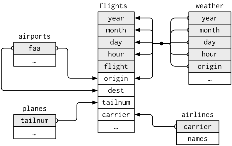 ] --- ## Your turn [Quiz 2](https://docs.google.com/forms/d/e/1FAIpQLSeQnfY6QXsXhIomcQ92dW70DSpYtZq-Yql4dlUvIUrE7FwYZg/viewform?usp=sf_link) 1. Imagine you wanted to draw (approximately) the route each plane flies from its origin to its destination. What variables would you need? What tables would you need to combine? --- ## Full solution [code](l05a/flights_join.R) --- ## Keys The variables that connect pairs of tables are called __keys__. A key is a variable (or set of variables) that uniquely identifies an observation. For example, each plane is uniquely identified by its `tailnum`, but identify an observation in `weather` you need five variables: `year`, `month`, `day`, `hour`, and `origin`. There are two types of keys: * A __primary key__ uniquely identifies an observation in its own table. For example, `planes$tailnum` is a primary key because it uniquely identifies each plane in the `planes` table. * A __foreign key__ uniquely identifies an observation in another table. For example, the `flights$tailnum` is a foreign key because it appears in the `flights` table where it matches each flight to a unique plane. --- class: code70 ## Keys The uniqueness of the keys is an invariant. Let's test it: ```r planes %>% count(tailnum) %>% filter(n > 1) ``` ``` ## # A tibble: 0 × 2 ## # … with 2 variables: tailnum <chr>, n <int> ``` ```r weather %>% count(year, month, day, hour, origin) %>% filter(n > 1) ``` ``` ## # A tibble: 3 × 6 ## year month day hour origin n ## <int> <int> <int> <int> <chr> <int> ## 1 2013 11 3 1 EWR 2 ## 2 2013 11 3 1 JFK 2 ## 3 2013 11 3 1 LGA 2 ``` .question[What happened at 1AM on November 3rd?] --- class: code70 ## Where's the primary key in `flights`? .pull-left[ Is he in the flight number? ```r flights %>% count(year, month, day, flight) %>% filter(n > 1) ``` ``` ## # A tibble: 29,768 × 5 ## year month day flight n ## <int> <int> <int> <int> <int> ## 1 2013 1 1 1 2 ## 2 2013 1 1 3 2 ## 3 2013 1 1 4 2 ## 4 2013 1 1 11 3 ## 5 2013 1 1 15 2 ## 6 2013 1 1 21 2 ## # … with 29,762 more rows ``` Nope. ] .pull-right[ Is he hiding in the plane tailnum? ```r flights %>% count(year, month, day, tailnum) %>% filter(n > 1) ``` ``` ## # A tibble: 64,928 × 5 ## year month day tailnum n ## <int> <int> <int> <chr> <int> ## 1 2013 1 1 N0EGMQ 2 ## 2 2013 1 1 N11189 2 ## 3 2013 1 1 N11536 2 ## 4 2013 1 1 N11544 3 ## 5 2013 1 1 N11551 2 ## 6 2013 1 1 N12540 2 ## # … with 64,922 more rows ``` Not here either. ] --- ## There he is! ```r flights %>% count(year, month, day, flight, origin, carrier) %>% filter(n > 1) ``` ``` ## # A tibble: 0 × 7 ## # … with 7 variables: year <int>, month <int>, day <int>, ## # flight <int>, origin <chr>, carrier <chr>, n <int> ``` It always pays to ask (but verify!) --- ## Surrogate keys If a table lacks a primary key, it's often useful to add one with `mutate()` and `row_number()`. That makes it easier to match observations if you've done some filtering and want to check back in with the original data. This is called a __surrogate key__. --- ## A tiny bit of database theory Tidy data sets will obey [various .alert[normal forms]](https://en.wikipedia.org/wiki/Database_normalization). The most basic is that there exists a .alert[primary keys] obeying a uniqueness and existence constraint. Highly normalized data sets also obey redundancy constraints that entail factoring (dividing) a data set into multiple tables. Unless you are a database engineer, complete normalization is often just a stumbling block to analyze data. However, it can be very helpful to think about dividing data into a primary table of **facts**, and auxiliary tables of **dimensions**. The facts represent frequently-updated observations and the dimensions are covariates that can be shared across observations and should change slowly, if at all.<sup>1</sup> .footnote[[1] See Kimball and Ross. *The Data Warehouse Toolkit* for details. It's surprisingly interesting and relevant.] --- # Class survey [How are things going so far?]( https://docs.google.com/forms/d/e/1FAIpQLSc2ThD_7Q9yCWJs5ucHpnVeDg9JougMe7shI__Wb332UmAVzg/viewform?usp=sf_link) --- # Acknowledgments Adapted from Data science in a box: [1](https://rstudio-education.github.io/datascience-box/course-materials/slides/u2-d09-tidying/u2-d09-tidying.html#1) [2](https://rstudio-education.github.io/datascience-box/course-materials/slides/u2-d08-multi-df/u2-d08-multi-df.html#1)